Schelling's Model of Racial Segregation

Racial residential segregation has existed for centuries and across different societies, often actively enforced by law. This was for example the case in the 19th century's United States with the Jim Crow laws. When the U.S. Supreme Court declared them unconstitutional in 1954, many expected segregation would disappear. This however was not the case: to the contrary, despite much effort and investment, segregation still remains a major issue in the U.S. and elsewhere to this date [1].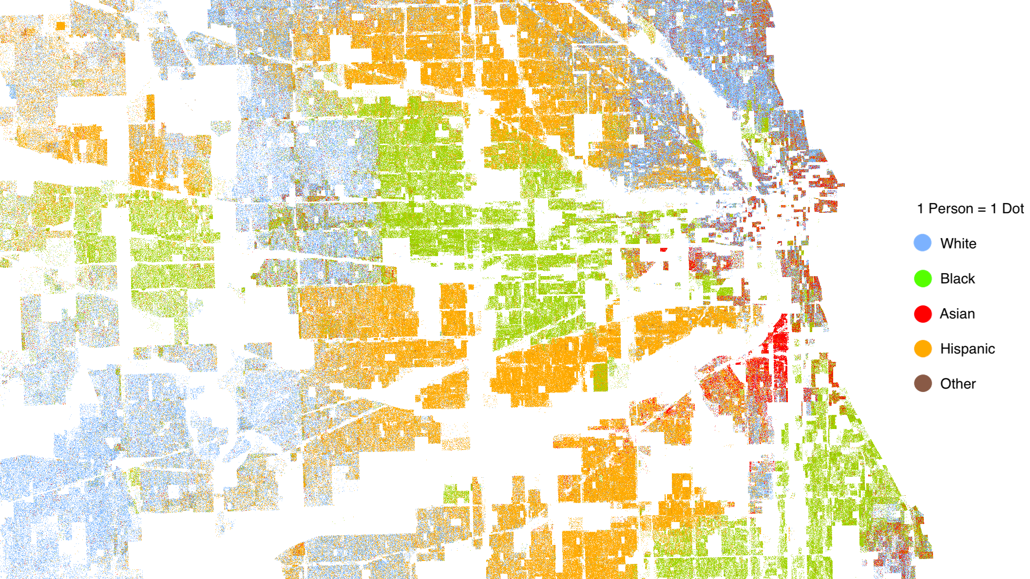



Even in absence of laws enforcing segregation, this can be caused by a number of factors including housing and loan discrimination, prejudice, etc. Yet another factor however, one which was not considered at the time, is that of emergence, that is the existence of macro-characteristics which are generated by the micro-level interactions of a complex system's constituents. In 1971, Thomas Schelling devised one of the earliest examples of agent-based models [3] suggesting that segregation could arise even when individuals would not mind being surrounded by different races, as long as they still desire to have at least a small fraction of people of the same racial background as neighbours. Despite the agents' willingness to accept a more diverse neighbourhood, segregation emerges nonetheless from the social interactions of different individuals. Strikingly, even weak local preferences can lead to major global phenomena emerging from the network of individual micro-interactions. Moreover, these emergent macro-regularities feed back onto the individual agents, constraining their choices and behaviour.

As we shall see, in spite of its simplicity, Schelling's model generates fascinating and complex dynamics, with multiple and far from intuitive equilibria.

A simple model of segregation

One of the simplest versions of Schelling's segregation model consists in a stylised representation of a residential area where individuals repeatedly make relocation decisions based on the characteristics of their immediate neighbourhood.
The model considers two types of agents, say blue and red, which might represent different races, ethnicities, economic status, etc., and a \(N\times N\) grid of residential locations over which a number \(N_a\le N^2\) of agents are initially randomly allocated. The agents' population is characterised by the fraction \(N_{b/r} = N_b / N_r\) of blue to red types such that \(N_a = N_b + N_r\), and assumed to be constant, so that at any given time one will have \(N_v = N^2 - N_a\) vacant residential locations. Each agent \(i\) is then characterised by a satisfaction parameter \(S_i\) given by the fraction of neighbours of the same type. Notice that the number of neighbours might depend on whether one considers fixed or periodic boundary conditions as well as on vacant locations which are not counted in the computation of \(S_i\).

Dynamics

The dynamics is set by a global tolerance parameter \(\tau\) denoting the maximum fraction of neighbours of a different type each agent is willing to accept before it decides to relocate. Therefore, every agent with \(S_i < 1 - \tau\) will relocate at random into a different vacant residential location. The dynamics continues until a stable equilibrium is found (if it exists) where all agents are satisfied.
As a consequence individuals' decisions are based exclusively on personal considerations based on the characteristics of the local neighbourhood they currently reside in. However, the act of relocation, despite being based on local parameters, ends up having global effect, since the random relocation of one agent might make discontent other agents which were previously satisfied.
Alternative versions of the model might consider a different behaviour whereby dissatisfied agents would move to the closest vacant location, instead of a random one, or to the best available location, or to the nearest location meeting the threshold \(1-\tau\). Yet another behavioural rule would allow individuals to move only if a better location is available. Notice that different rules might have important repercussions on global dynamics. Consider as an example the version in which all dissatisfied individuals move at random (which is what we shall employ hereafter). Clearly for sufficiently low tolerance \(\tau\) and/or sufficiently low rate of vacant properties no static equilibrium will exist, since there will always be at least one individual unsatisfied with its location and unable to find another suitable one. On the other hand a static equilibrium always exist when considering individuals relocating only if a better location is found.

Simulations

In the following we employ a Python implementation of Schelling's segregation model on an \(N\times N\) grid with \(N=60\), assuming \(10\%\) of all properties being vacant at any given time, a \(1\)-to-\(1\) ratio of red to blue agents. Let us start by defining the system's parameters:

N = 60       # Grid will be N x N
SIM_T = 0.4  # Similarity threshold (that is 1-τ)
EMPTY = 0.1  # Fraction of vacant properties
B_to_R = 1   # Ratio of blue to red people

Although objected-oriented programming is often the favoured programming paradigm in agent-based modelling, this might not be the most suitable approach when looking for numerically efficient routines. Therefore, in order to maintain high efficiency in the simulations we shall model the system as a numpy.array of size (N, N), encoding residential locations occupied by blue agents as 0, those occupied by red agents as 1, and vacant properties as -1.
Now one needs two main functions: a rand_init function for the random initialisation of the system matrix M, and a evolve function to impose on the system the dynamics described above. The former is easily implemented as

import numpy as np

def rand_init(N, B_to_R, EMPTY):
    """ Random system initialisation.
    BLUE  =  0
    RED   =  1
    EMPTY = -1
    """
    vacant = N * N * EMPTY
    population = N * N - vacant
    blues = int(population * 1 / (1 + 1/B_to_R))
    reds = population - blues
    M = np.zeros(N*N, dtype=np.int8)
    M[:reds] = 1
    M[-vacant:] = -1
    np.random.shuffle(M)
    return M.reshape(N,N)

The following Fig. 3 presents as example of a randomly initialised system, with the parameters specified above.

The evolution function instead is where most of the computational effort lies, and more specifically in the computation of the satisfaction parameters \(S_i\). For a fast implementation we can rely on convolution of the matrix M with the kernel

KERNEL = np.array([[1, 1, 1],
                   [1, 0, 1],
                   [1, 1, 1]], dtype=np.int8)

The convolution operation on a kernel \(K\in\mathbb{R}^{(2k_x+1)\times (2k_y+1)}\), with \(k_x, k_y \in\mathbb{N}_0\), is defined as Therefore, each element of the convolution \(K\star M\) contains the sum of all neighbouring values.
With this in mind, we can now write a function to take care of the dynamical evolution of the system:

from scipy.signal import convolve2d

def evolve(M, boundary='wrap'):
    """
    Args:
        M (numpy.array): the matrix to be evolved
        boundary (str): Either wrap, fill, or symm
    If the similarity ratio of neighbours
    to the entire neighbourhood population
    is lower than the SIM_T,
    then the individual moves to an empty house.
    """
    kws = dict(mode='same', boundary=boundary)
    B_neighs = convolve2d(M == 0, KERNEL, **kws)
    R_neighs = convolve2d(M == 1, KERNEL, **kws)
    Neighs   = convolve2d(M != -1,  KERNEL, **kws)

    B_dissatified = (B_neighs / Neighs < SIM_T) & (M == 0)
    R_dissatified = (R_neighs / Neighs < SIM_T) & (M == 1)
    M[R_dissatified | B_dissatified] = - 1
    vacant = (M == -1).sum()

    N_B_dissatified, N_R_dissatified = B_dissatified.sum(), R_dissatified.sum()
    filling = -np.ones(vacant, dtype=np.int8)
    filling[:N_B_dissatified] = 0
    filling[N_B_dissatified:N_B_dissatified + N_R_dissatified] = 1
    np.random.shuffle(filling)
    M[M==-1] = filling

Notice that the boundary argument of scipy.signal.convolve2d provides an easy way to switch from fixed ('fill') to periodic ('wrap') boundary conditions. In the following we shall stick to the latter.

Finally we are able to run simulations: Fig.4 shows the evolution from a randomly initialised state with a high degree of integration towards a segregated configurations where each region is separated by a layer of vacant locations. Notice that because of the periodic boundary conditions, the reds almost form a single blob, with the exception of a small island in the center left of the computational grid and similarly for blue agents.

Unsurprisingly, large levels of intolerance lead to fully segregated configurations. What is unexpected however, is the degree of segregation that naturally emerges even for seemingly low levels of intolerance. Even when individuals are willing to accept up to \(60\%\) of diverse neighbours (\(1-\tau=0.4\)), one would still observe segregation emerging, as shown in Fig. 5 below. Put differently, and this is one of the main insights of Schelling, aggregate segregation can emerge even just from the desire of individual’s not to feel in an extreme minority. The interaction between the decisions of different agents with such an arguably weak requirement on the composition of their residential neighbourhood is sufficient to lead to the emergence of segregation. The self-reinforcing mechanism driving the emergence is found in increased likelihood of individuals in a neighbourhood to relocate conditional on one individual relocating. When a minority individual leaves a neighbourhood, that type of agent becomes rarer in that neighbourhood, therefore providing an incentive for others to move as well.

The degree of segregation can be measured by the mean satisfaction \(\langle S\rangle\) over the population of individuals. As discussed, this increases up to a critical threshold after which the system becomes unstable and no static equilibrium can be found (see Fig. 6). Moreover, up to the critical threshold, that is when a static equilibrium exists, one systematically observes \(\langle S \rangle_{\text{eq}} \ge 1-\tau\). Notably, the mean satisfaction \(\langle S\rangle\) is quantised with discrete transitions occurring at specific values of the preference \(1-\tau\).

The quantisation of \(\langle S\rangle\) can be traced to the discreteness of the neighbourhood of each individual (Fig. 7). Neglecting vacant locations each individual can have at most \(8\) neighbours which might or might not be of the same type. Consequently, quantised jumps in \(\langle S\rangle\) can be expected to occur at any \(\frac{n}{8}\) for \(n∈ℕ:n<8\).

Naturally, with an increasing fraction of vacant locations a finer quantised structure emerges, as the expected number of neighbours decreases (recall that vacant places do not count towards the computation of \(S_i\)). Thus, more generally, one can expect to find quantised jumps in \(\langle S\rangle\) at \(\frac{n}{m}\) for \(n,m∈ℕ:m\le 8, n < m\). These fractions are marked by red vertical lines in Fig. 7 above; higher lines correspond to higher values of \(m\).

References

[1] "Racial Segregation Is Still a Problem", Michael Cassidy, The Century Foundation, July 2013
[2] "The Racial Dot Map", Demographics Research Group, Weldon Cooper Center for Public Service, University of Virginial, 2017
[3] "Dynamic Models of Segregation", Thomas C. Schelling, Journal of Mathematical Sociology, 1971, Vol.1, pp143-186

Back to Teaching

---